What is ocean acidification?
Acidification is defined as an increase in the concentration of H + in a solution or a lowering of a solution’s pH. Ocean acidification is therefore the reduction of the pH of the world’s oceans.
This can occur when CO2 dissolves in water and there is a reaction between the H2O andCO2 to form carbonic acid (H2CO3).
[CO2] + [H2O] <=> [H2CO3]
This weak acid readily releases a proton (H+) and a negatively charged inorganic carbon ion.
[H2CO3] <=> [H+] + [HCO3-]
The release of the H+ into the water will make it more acidic, that is it will drive the pH down. This increase in H+ will also react with the carbonate ion (CO32-) to form HCO3-
[H+] + [CO32-] <=> [HCO3-]
The overall effect of CO2 dissolving into water is that the concentrations of H+, H2CO3 and HCO3- increase and the concentration of CO32- decreases and the solution is more acidic (i.e. a decrease in pH. The world’s oceans readily exchange CO2 with the atmosphere. As the concentration of CO2 in the Earths atmosphere increases, so to does the level of CO2 that the oceans absorb and therefore increasing the concentrations of H+ in the ocean making them more acidic.
What is causing ocean acidification?
As carbon dioxide obeys Henry’s Law (which states that the concentration of a dissolved gas in a solution is directly proportional to the partial pressure of that gas above the solution) an increase in the concentration of CO2 in the atmosphere directly leads to an increase in the amounts of CO2 absorbed by the oceans. Human induced CO2 emissions have increased since the industrial revolution through the burning of fossil fuels, land use practices and concrete production((Antarctic Climate and Ecosystems Cooperative Research Centre (2008). Position analysis: CO2 and climate change, ocean impacts and adaptation issues. Hobart, TAS.)). This increase from around pre-industrial values of 280 parts per million (ppm) to 383ppm today (See Enhanced Greenhouse Effect) has resulted in the acidification of the ocean.
![The averaged CO2 concentrations measured at Cape Grim Tasmania from 1975-2005 [2]. Reprinted with Permission from CSIRO and Bureau of Meteorology.](/wp-content/uploads/2016/09/oze_fs_004_02.gif "The averaged CO2 concentrations measured at Cape Grim Tasmania from 1975-2005 [2]. Reprinted with Permission from CSIRO and Bureau of Meteorology.")
Figure 1. The averaged CO2 concentrations measured at Cape Grim Tasmania from 1975-2005((CSIRO Cape Grim Website – http://capegrim.csiro.au/.)). Reprinted with Permission from CSIRO and Bureau of Meteorology.
The rate of increase is far greater than generally occurs naturally and is predicted to continue to rise well into the future((IPCC (2007). The Fourth assessment report of the Intergovernmental Panel on Climate Change (IPCC). Climate Change 2007: The Physical Science Basis. (Solomon, S., D. Qin, M. Manning, Z. Chen, M. Marquis, K.B. Averyt, M. Tignor and H.L. Miller, Editors). Contribution of the Working Group I to the Fourth Assessment Report of the Intergovernmental Panel on Climate Change. Cambridge University Press, 944pp.)). Approximately 25% of the CO2 from burning fossil fuels and cement production in the past 200 years has already been absorbed by the oceans. This CO2 absorption has already led to a decrease in the pH of the oceans of about 0.1 units from pre industrial levels. While this value seems very small, this is mostly an artefact of the way that pH is measured. Put another way this change represents about a 30% increase in the concentration of H+ in seawater. More importantly the H+ concentration, and the rate at which it is rising, are both still increasing((The Royal Society (2005) Ocean Acidification due to increasing atmospheric carbon dioxide. Science Section, The Royal Society, London.)).
What is the significance of Ocean Acidification?
Bioavailability of carbonate
Many marine organisms make shells or supporting plates out of calcium carbonate (CaCO3) in a process called calcification. As water becomes more acidic, the calcification process is inhibited and the growth and/or survival of certain organisms could be affected. As many of these organisms form the primary production of oceans, any change in their life cycle has the potential to impact all marine ecosystems.
 and dissolved CO2 concentration (dashed lines) for average surface waters in the tropical ocean (thick lines), the Southern Ocean (thickest lines) and the global ocean (thin lines)")
Figure 2. Shown are both CO32- concentration (solid lines) and dissolved CO2 concentration (dashed lines) for average surface waters in the tropical ocean (thick lines), the Southern Ocean (thickest lines) and the global ocean (thin lines). Solid and dashed lines were calculated from the thermodynamic equilibrium approach. For comparison, open symbols are for CO32- concentration from a non-equilibrium, model-data approach versus seawater pCO2 (open circles) and atmospheric pCO2 (open squares); symbol thickness corresponds with line thickness, which indicates the regions for area-weighted averages. The nearly flat, thin dotted lines indicate the CO32- concentration for seawater in equilibrium with aragonite (aragonite saturation) and calcite (calcite saturation). Reprinted by permission from Macmillan Publishers Ltd: Nature, Orr et al. 2005((Orr J. C., Fabry V. J., Aumont O., Bopp L., Doney S. C., Feely R. A., Gnanadesikan A., Gruber N., Ishida A., Joss F., Key R. M., Lindsay K., Maier-Reimer E., Matear R., Monfray P., Mouchet A., Najjar R. G., Plattner G. K., Rodgers K. B., Sabine C. L., Sarmiento J. L., Schlitzer R., Slater R. D., Totterdell I. J., Weirig M. F., Yamanaka Y. and Yool A. (2005) Anthropogenic ocean acidification over the twenty first century and its impact on calcifying organisms . Nature 437, 681-686)).
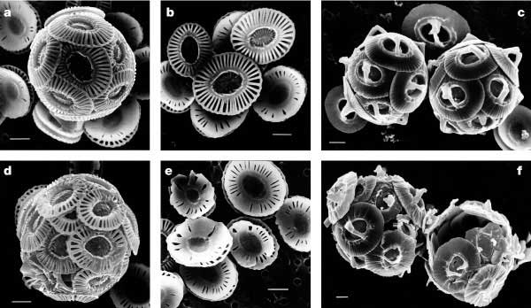
Figure 3. The impact of higher than current CO2 concentration on the calcification of coccolithophorids. Shells a, b, d, e, are Emiliania huxleyi ; and shells c, f, are Gephyrocapsa oceanica. Shells in the top 3 images were grown at slightly above pre-industrial CO2 levels (incubated at [CO2] ≈ 12 µ mol l -1, pCO2 levels of 300 ppmv) and those in the bottom 3 images were grown around three times pre-industrial levels (incubated at [CO2] ≈ 30–33 µ mol l -1, p CO2 levels of 780–850 ppmv). Scale bars represent 1 µ m. Reprinted by permission from Macmillan Publishers Ltd: Nature, Riebesell et al. 2000((Riebesell, U., Zondervani, I. , Rost, B., Tortell, P.D., Zeebe, R. and Morel, F.M.M. (2000) Reduced calcification of marine plankton in response to increased atmospheric CO2. Nature 407, 364-367.)).
The Southern Ocean has been identified as being particularly vulnerable to becoming under saturated in calcium carbonate as it already has very low saturation levels((IPCC (2007). The Fourth assessment report of the Intergovernmental Panel on Climate Change (IPCC). Climate Change 2007: The Physical Science Basis. (Solomon, S., D. Qin, M. Manning, Z. Chen, M. Marquis, K.B. Averyt, M. Tignor and H.L. Miller, Editors). Contribution of the Working Group I to the Fourth Assessment Report of the Intergovernmental Panel on Climate Change. Cambridge University Press, 944pp.)). The saturation level of the carbonate minerals is not only dependent on the concentrations of dissolved CO2 and carbonate but also with water temperature and pressure. The solubility of CaCO3 increases with decreasing temperature and increasing depth (See Carbonate Buffering). However, with increasing dissolved CO2 concentrations the depth at which the CaCO3 minerals will become under saturated will rise, i.e. the depth at which CaCO3 minerals will begin to dissolve (particularly the more soluble mineral form- Aragonite) will become shallower. This saturation depth is predicted to reach the surface in some areas of the Southern Ocean if CO2 levels rise to twice their current levels, which could have a significant impact on the marine food webs on Australia ‘s southern coastline((Orr J. C., Fabry V. J., Aumont O., Bopp L., Doney S. C., Feely R. A., Gnanadesikan A., Gruber N., Ishida A., Joss F., Key R. M., Lindsay K., Maier-Reimer E., Matear R., Monfray P., Mouchet A., Najjar R. G., Plattner G. K., Rodgers K. B., Sabine C. L., Sarmiento J. L., Schlitzer R., Slater R. D., Totterdell I. J., Weirig M. F., Yamanaka Y. and Yool A. (2005) Anthropogenic ocean acidification over the twenty first century and its impact on calcifying organisms . Nature 437, 681-686)).
![The change in CO332- ([CO32-]A) is the in situ [CO32-] minus that for aragonite-equilibrated sea water at the same salinity, temperature and pressure](/wp-content/uploads/2016/09/oze_fs_004_07.jpg "The change in CO332- ([CO32-]A) is the in situ [CO32-] minus that for aragonite-equilibrated sea water at the same salinity, temperature and pressure")
Figure 4. The change in CO332- (Δ[CO32-]A) is the in situ [CO32-] minus that for aragonite-equilibrated sea water at the same salinity, temperature and pressure. Shown are the OCMIP-2 median concentrations in the year 2100 under scenario IS92a: a , surface map; b , Atlantic; and c , Pacific zonal averages. Thick lines indicate the aragonite saturation horizon in 1765 (Preind.; white dashed line), 1994 (white solid line) and 2100 (black solid line for S650; black dashed line for IS92a). Positive Δ[CO32-]A indicates supersaturation; negative Δ[CO32-]A indicates undersaturation. Reprinted by permission from Macmillan Publishers Ltd: Nature, Orr et al. 2005((The Royal Society (2005) Ocean Acidification due to increasing atmospheric carbon dioxide. Science Section, The Royal Society, London.)).
Speciation of Nutrients
The speciation, or the ionic form, of compounds is dependant on a number of factors such as their concentration, the presence or absence of other ions and pH . For example, in seawater phosphate can be present as PO43-, HP0442-, H2PO4- and H33PO4 depending on what the pH of the solution is. Theoretical speciation diagrams predict that the speciation of nutrients such as phosphate, silicate, iron and ammonia would all be impacted within the range of pH decreases predicted((Zeebe and Wolf-Gladrow (2001) )). For example as pH decreases ammonia (NH3) concentrations would be lowered in preference to the ammonium species (NH4+).

Figure 5. Changes in speciation of phosphate, silicate and ammonia with pH. The red box shows the range that pH is predicted to change within. Reprinted with permission form Zeebe and Wolf-Gladrow 2001((Zeebe and Wolf-Gladrow (2001) )).
The speciation of ions could affect their bioavailability. For example the ratio of soluble to insoluble iron may be increase making iron more available and reducing the growth limiting effect that low soluble iron concentrations have in some areas. The low availability of soluble iron has been shown to limit the growth of phytoplankton in the Southern Ocean and by artificially increasing soluble iron concentrations there is an increase in photosynthetic activity and phytoplankton biomass((Boyd P. W., Watson A. J., Law C. S., Abraham E. R., Trull T., Murdoch R., Bakker D. C. E., Bowie A. R., Buesseler K. O., Chang H., Charette M., Croot P., Downing K., Frew R., Gall M., Hadfield M., Hall J., Harvey M., Jameson G., LaRoche J., Liddicoat M., Ling R., Maldonado M. T., McKay R. M., Nodder S., Pickmere S., Pridmore R., Rintoul S., Safi K., Sutton P., Strzepek R., Tanneberger K., Turner S., Waite A. and Zeldis J. (2000) A mesoscale phytoplankton bloom in the polar Southern Ocean stimulated by iron fertilization. Nature 407, 695-702)).
 and the measured solubility (b) of Fe(III) in seawater as function of pH")
Figure 6. The speciation (a) and the measured solubility (b) of Fe(III) in seawater as function of pH. From Millero 1998((Millero F. J. (1998) The solubility of Fe(III) n seawater. Earth and Planetary Science Letters 154 (1-4) 323-329)).
However, changes to metals speciation, could possibly allow for more free dissolved heavy metals and an associated increased toxicity effect.
Changes to biodiversity
Some species will be better suited to higher CO2 and lower pH and a shift from one set of dominant species to another could have a huge impact on the entire ecosystems. For example animals such as deep sea fish and cephalopods are particularly sensitive to external CO2. Squid are seen as sensitive due to their energy intensive form of movement. This extremely active use of muscles requires a large supply of oxygen. However, the capacity of blood to carry oxygen can be reduced by high CO2 levels. At this stage it is unclear what impacts the levels of CO2 predicted for the next 100 years would have on the life cycles of multicellular organisms((IPCC (2007). The Fourth assessment report of the Intergovernmental Panel on Climate Change (IPCC). Climate Change 2007: The Physical Science Basis. (Solomon, S., D. Qin, M. Manning, Z. Chen, M. Marquis, K.B. Averyt, M. Tignor and H.L. Miller, Editors). Contribution of the Working Group I to the Fourth Assessment Report of the Intergovernmental Panel on Climate Change. Cambridge University Press, 944pp.)).
Considerations for measurement and interpretation
Predicting Atmospheric CO2
While the absorption of CO2 by seawater is defined by Henry’s Law, there is no such certainty about the future levels of CO2 in the atmosphere. For the IPCC Fourth Assessment report the projections of CO2 emission are based on a number of scenarios which outline future patterns of economic growth, fossil fuel dependence and technology development((IPCC (2000). Special Report on Emission Scenarios. A Special Report of Working Group III of the Intergovernmental Panel on Climate Change. Cambridge University Press, Cambridge, UK)). These projections forecast CO2 reaching levels of between 550 ppm to 850-970 ppm by the year 2100. The lower value assumes a strong uptake of clean and efficient technology across the globe with the higher value resulting from a continued and increased worldwide dependence on fossil fuels. The rate at which atmospheric CO2 concentrations increase will dependent on economic development, technology advancement and societal pressures along with several environmental processes and all these will need to be accounted for in future models used to predict ocean acidification.
An example of an environmental process in the carbon cycle is calcification, which releases CO2.
2[HCO33-] + Ca2+ <=> [CaCO3] + [H2O] + [CO2]
It is unclear how acidification, and any associated restriction of calcification, might be offset by the decrease in CO2 released by calcification. Zondervan et al.((Zondervan I, Zeebe R E, Rost B & Riebesell U (2001) Decreasing marine biogenic calcification: a negative feedback on rising atmospheric pCO2. Global Biogeochemical Cycles 15, 507-516)) estimate that with increasing atmospheric CO2, CO2 emitted by the oceans could increase from 0.63 Gt of carbon per year in 1850 to 0.85 Gt per year by 2150. However, they assumed a constant rate of calcification which would not be the case if calcification was inhibited by increasing acidity. Also with decrease in the amount of CO2released during carbonate production, the oceans would have lower dissolved CO2concentrations and be able to absorb more CO2from the atmosphere((Riebesell, U., Zondervani, I. , Rost, B., Tortell, P.D., Zeebe, R. and Morel, F.M.M. (2000) Reduced calcification of marine plankton in response to increased atmospheric CO2. Nature 407, 364-367.)).
Carbonate Buffering
As CO2levels in the atmosphere increase and there is a increase in H+ and a decrease in CO3-2, the depth below the surface of the ocean at which CaCO3 becomes supersaturated (below which CaCO3 will become under saturated and therefore dissolves) will become shallower. This would result in some currently mineralised CaCO3 deposits dissolving and releasing carbonate ions.
[CaCO3] + [H2CO3] <=> [Ca2+] + 2[HCO3-]
Note that this reaction would utilise the carbonic acid resulting from increased CO2 absorption and decrease the level of acidification produced. This natural process, called buffering, acts to continuously stabilise the pH of seawater. The work that has been done to model the extent to which ocean acidification will affect the carbonate saturation depth, and how changes to that depth will modify the capacity of seawater to buffer any increases in H+ concentrations, suggests that that the process will be very slow and not fast enough to offset the rapid acidification from CO2 absorption((Caldeira K. and Wickett M. J. (2003) Anthropogenic carbon and ocean pH. Nature 425, 365)).
Temperature and Circulation Effects
Temperature and pressure (water depth) both have an impact on the solubility of CO2 and CaCO3 in seawater. Sea surface temperatures (SST) also impact on ocean circulation and mixing which will affect the rate and extent to which any changes to seawater pH will occur. It is unclear at this time how any increases in SST and or changes to oceanic circulation associated with climate change might enhance or ease the overall ocean acidification effect of increased CO2 in the earth’s atmosphere.
Existing information and Data
Little research has been done to investigate the potential impacts of ocean acidification, and even less on these might manifest in estuaries and coastal areas.
Key questions and further research needs
- The identification of the species and ecosystems most sensitive to increased CO2
- The interaction between increased CO2 and other factors such as water temperature, sediment process, changed runoff patterns and carbon cycles and nutrient cycles, speciation of trace metals and particle flocculation.
- Identification of estuaries that would be most sensitive to impacts of ocean acidification
Authors
- Geoscience Australia
- Department of Climate Change